Introduction

Demand estimation is the process of forecasting, with varying levels of confidence and accuracy, the sources, amounts, and timing of production demand by consumers. It involves analyzing past data and trends to predict demand as well as gathering forecasts from customers to inform the model as well.

Multiple business units have an interest in reliable, accurate, and timely forecasts. Business leadership relies on long-term forecasts to manage infrastructure and resources such as manufacturing facilities or relationships. Financial groups use revenue and gross profit forecasts to project cash flow and cash runway or to time investment rounds. Sales and marketing often provide and maintain the inputs to the demand estimation records and adjust their models from realized sales. Even production planners can look to near-term estimates as a sign of what is likely to come and adjust production schedules or safety stock accordingly.

Primary Roles of Demand Estimation

The demand estimation tool should not be confused with the material resource planning workflow for determining component shortages for your production schedule. The primary roles of the demand estimation tool are:

1. Provide a way in which you can enter and maintain your product demand estimates (i.e. customer demand). Alone, this can be useful to help understand your financial sales forecasts.
2. Aggregate component demand forecasts. This can be helpful when communicating forecasts to vendors, but note that these shouldn’t be necessarily considered “actionable”. Demand estimates have a corresponding prominence attribute which can help your organization understand the level of confidence in each product demand estimate and, therefore, the resulting component demand estimates. These component demand estimates are more useful for telling vendors something like “We’re expecting to use about 50,000 of these parts through the next 5 years, growing to eventually about 18,000 per year.”
3. Providing balance to the production schedule. If you have a production schedule to produce 1,000 units of some product every 3 months, your forecast inventory will simply grow unbounded because outflow inventory isn’t there to balance it. Demand estimates provide a way for you to balance this and forecast for safety stock targets and tune your production schedule.

Actionable and Non-Actionable Demand

Demand estimation is an exercise in nuance. The entire organization must agree on the meaning and actionability of a particular estimate. For example, if component lead times are 2 to 3 months, a three year forecast is not likely actionable for a production planner, but may be actionable for a business leader who must take steps to build a manufacturing facility that will take two years to complete.

Fundamentals of Demand Estimation

Demand Entries

The demand entry is the basic unit of demand estimation. Each demand entry represents a potential sales opportunity within the context of MRP, production planning, and inventory management with the following attributes:

• Item Number (i.e. Manufacturer Part Number)
• Quantity
• Date – When in the future the consumption is expected to take place
• Consumer – A specific customer or channel (e.g. Amazon, eCommerce, distributor)
• Warehouse – Where the consumption takes place (e.g. Headquarters, Finished Goods)
• Revenue (optional) – Used to formulate a revenue forecast model
• Prominence – A “grouping” of similarly likely demand that can be used to determine actionability

Spot Demand and Flow Demand

Demand entries may be singular (spot demand) to represent a single opportunity or they may be grouped as a collective (flow demand) to make it easier to describe and manage growth or declining trends over a period of time.

Example 1: Spot Demand

Your sales team is working with a customer on a one-time purchase of vehicles to satisfy their demand for a new fleet site in Oklahoma. The opportunity is for 150 vehicles produced in the Bloomington, Illinois manufacturing facility with an expected delivery date of 2025-06-15.

Example 2: Flow Demand

Your company is about to release a new high-end network router. Over the expected 6 year lifecycle of the product, it is expected to go through three phases: growth, sustain, and phase-out. Each phase will last two years and your team describes each phase as 8 demand entries, each representing a quarter. In the growth phase, demand increases from 100 units by 25 units per quarter (100, 125, 150, …, 275). In the sustain phase, demand is expected to increase by 5% each quarter (288, 303, 318, and so on). In the phase-our, demand is expected to decrease by 20% each quarter.

Product Demand Forecast

The collection of demand entries is aggregated in the product demand matrix to show each product’s demand for a specific period of time for planning and reporting purposes. Revenue, gross profit, and customer breakdowns can be useful for financial forecasts and investor relations.

Component Demand Forecast

With demand entries established, component demand is determined by collecting the derivative demand for each component from all assemblies. Again, noting that this is a forecast and not necessarily actionable for procurement purposes, component demand can provide important insights to buyer/planners. For example:

• Sharing component forecasts with vendors for specific manufacturers, families, or types of products can help negotiate long-term pricing contracts.
• Product lifecycle planning is influenced by the lifecycle of components on the products. Understanding forecast demand is crucial to understanding the impact that lifecycle changes on components will have to the product portfolio.
• Engineering of new products can also benefit from demand forecasts when deciding whether or not to incorporate an existing database part that may have otherwise declining forecasts or to pick up an alternative that has a brighter outlook.

Inventory Forecasting

An inventory forecast chart is an effective tool for balancing production and demand, offering a visual representation of a company’s current and projected inventory levels. In the absence of demand (outgoing inventory due to sales activities), inventory will increase without bound based on the production schedule.

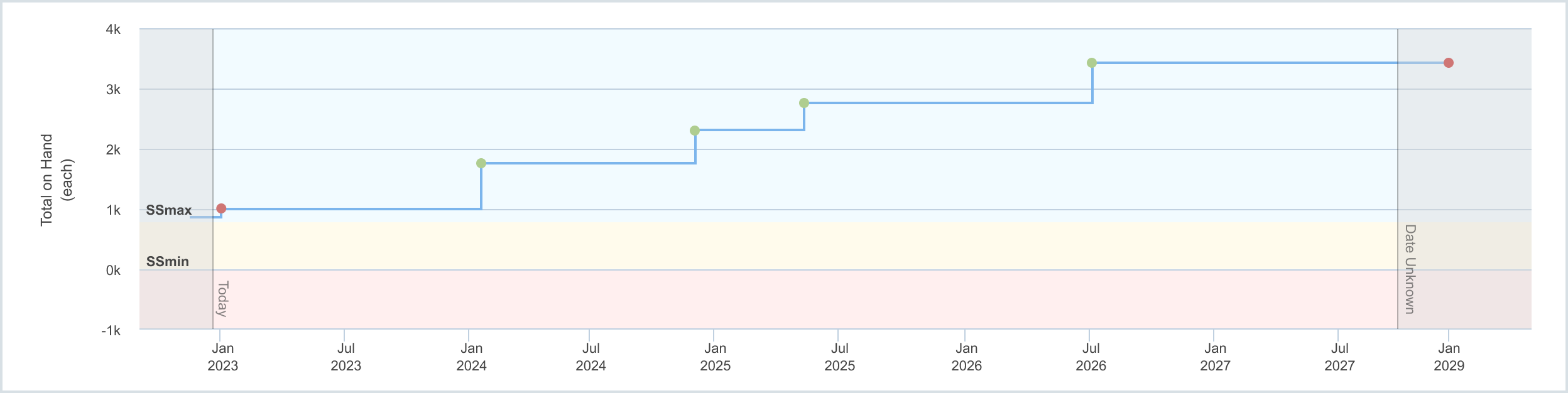
By including demand forecasts, the inventory forecast chart becomes a more useful tool for estimating inventory levels into the future. Production events (such as batch builds) are represented as an increase in inventory. Sales events (demand entries) are represented as a decrease in inventory.

In the example above, safety stock ranges are represented with the red, yellow, and blue colored bands. Using the chart as a guide, planners can identify periods when production needs to be increased to meet customer demand and when it should be reduced to prevent overstocking.

Integrating with a Sales Funnel

Product demand estimates are typically generated by the marketing and sales team. For a new product introduction (NPI), there may be early adoption customers that purchased previous generations of the product, channels that are eager to introduce a new technology to waiting customers, or the product may be completely speculative with a lot more uncertainty in demand. After a product is released, the sales funnel gains certainty and volume at the lower end with new opportunities entering at the top.

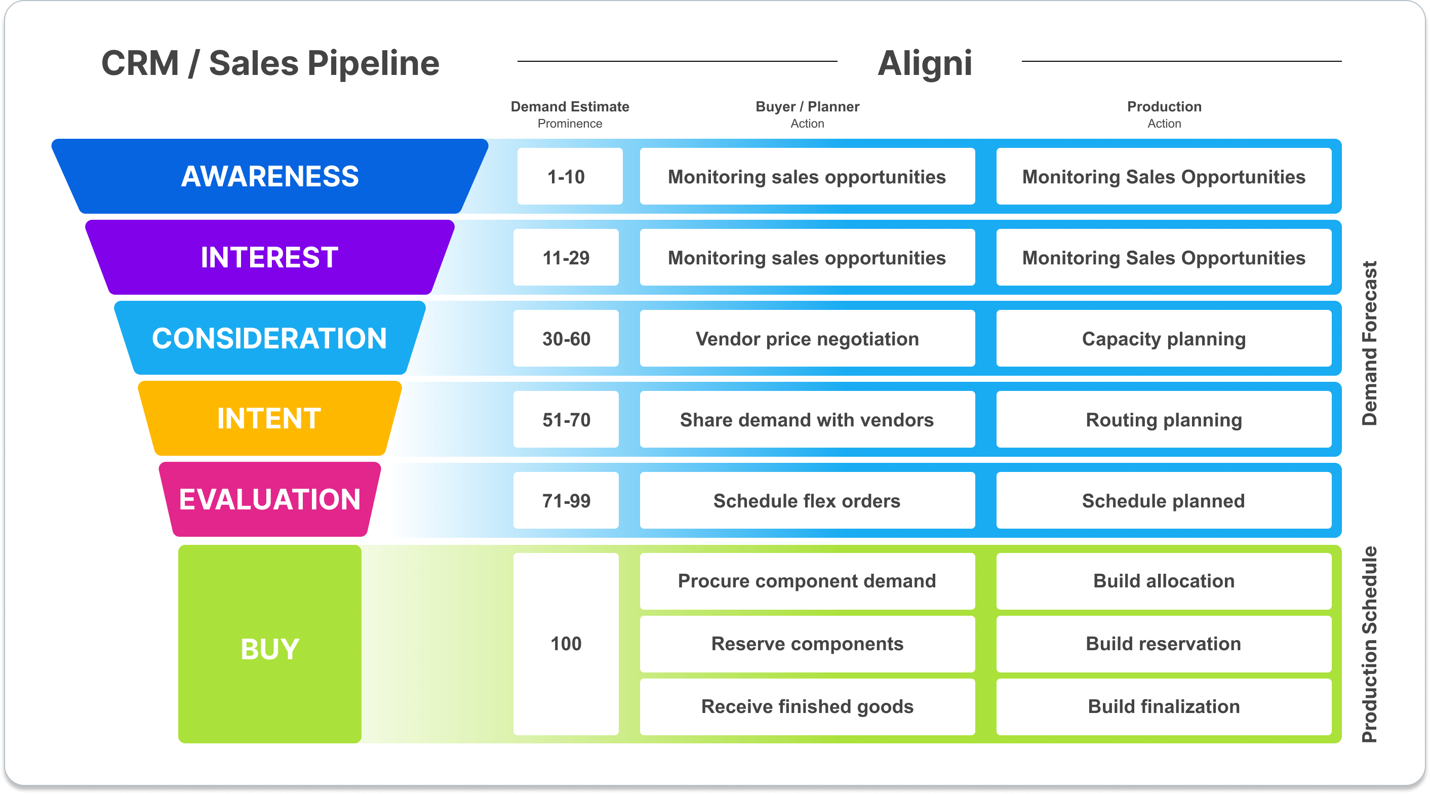
Depending on where an opportunity has progressed within the sales funnel, it may influence different activities among other groups, ultimately resulting in component procurement and production. This final stage is represented in the MRP Workflow. Aligni’s MRP Workflow is a world of certainties, so we have introduced the notion of demand prominence to relate stages of confidence in the sales funnel to activities within the planning and production team.

Demand Prominence

It is common for sales and marketing to attribute a confidence number (sometimes described as a percentage, but much less mathematically dependable as such) to a particular opportunity. These opportunities are represented as demand estimates in Aligni with a prominence number (we do not refer to them as a percentage, but if it makes you more comfortable to do so, you may!). In the chart above, we have shown some ranges for prominence that might be appropriate, but your organization should establish your own rules and align them across business units.

Using prominence as a mask to effectively hide demand entries below some established prominence offers a way to consider only demand estimates that meet some confidence threshold. For example, when planning ahead to manage future safety stock levels, buyer/planners may want to consider demand over some specific threshold depending on the cost, lead time, lifecycle status, or other parameters for the item under evaluation.

Here’s an example demand prominence schedule that an organization may use to align sales, finance, and production departments with the prominence meanings:

Prominence	Sales	Finance	Production	Notes
100	Placed Orders	Forecast	Actionable	Orders placed but still pending payment and production. These should be high confidence (near certainties). These are attributed to a specific customer.
90	eCommerce (est)	Forecast	Actionable	eCommerce forecasts are based on estimates of sales velocity and reflect a combination of order history and any other factors that influence the forecast. They are attributed to the eCommerce channel and not any specific customer.
70	High-Q Customer Forecast	Forecast	Non-Actionable	Planned orders or forecasts from reliable customers with approved or active programs. These customers have generally proven themselves to be reliable at forecasting and dependable. These are included in financial estimates (P&L). Production may use this demand for low-cost components but not high-cost components (e.g. FPGAs) or production (builds).
50	Demoted	None	None	This is a previously reliable forecast that has been demoted after some period of no communication with the customer.
10	Low-Q Customer Forecast	None	None	Early conversations with customers representing low-quality forecasts. Often these will represent a project that has not yet been approved or completed.

Buyer/Planner Activities

Buyer/planner activities based on demand estimates are a function of the confidence (prominence) as well as the risk tolerance of the organization. Some low-cost components may be ordered based on lower prominence demand, whereas high-value components may be ordered only when a customer PO is secured.

Even before component procurement, however, buyer/planners can use lower-prominence demand in negotiations and discussions with vendors or when placing scheduled, recurring, or blanket orders with some flexibility in quantity or delivery timing.

Production Activities

Similarly, most production activities will only be initiated on a secured customer PO. However, some long-term planning and operations may lean on weaker demand estimates if they are accompanied by a long lead time. Building out additional capacity or facility capabilities may be justifiable if the organization needs to take risks in a particularly competitive environment, for example.

Revenue Modeling

Sales estimates may also be used to construct revenue models for financial planning. Since these estimates have some level of underlying uncertainty, statistical models can be incorporated into each estimate for basic reporting or more elaborate confidence-based outcomes using Monte Carlo analysis.

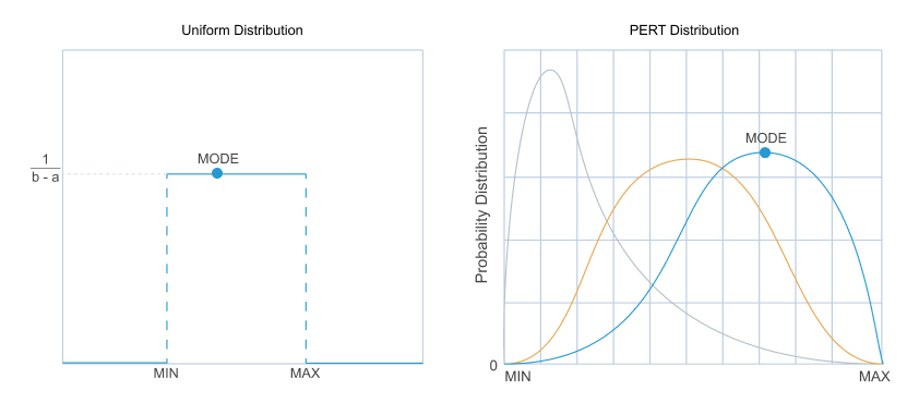
Two common distribution models that may be used for such estimates are the uniform distribution and PERT distribution, shown below.

In the uniform distribution, all values between the minimum and maximum specified quantity are equally likely. While there is not any “maximally likely” value (mode), setting a specific value can still be helpful for non-statistical analysis.

The PERT distribution approximates a Gaussian distribution (bell curve) but with two helpful qualities. First, whereas a Gaussian distribution is infinite, there is no long tail to the PERT distribution so that it fits neatly between the minimum and maximum. Second, the mode may be set at any point between min and max to bias the distribution. These qualities make the PERT distribution well-suited to demand estimation.

Documentation

To learn more about Aligni’s demand estimation capabilities and how to deploy them, please visit our online documentation page.